Test Quiz 13

Two different brands of tablets with the same active compound are compared with respect to their solubility. For each of the two brands 10 tablets were investigated. For each tablet, percent solubility is measured after the tablet have been kept in 1000 ml de-ionized water for a while. One measurement failed, so the following values for percent solubility were found:

Brand F	45	47	48	49	49	50	52	52	53	54
Brand G	48	48	49	49	52	54	54	55	55

A 99% confidence interval for the difference between the two means, which is not based on an assumption about normality of the data, is wanted. The following Python code is executed:

x = np.array([45, 47, 48, 49, 49, 50, 52, 52, 53, 54])   y = np.array([48, 48, 49, 49, 52, 54, 54, 55, 55])

k = 10000 xsamples = np.random.choice(x, size=(len(x), k), replace=True) ysamples = np.random.choice(y, size=(len(y), k), replace=True) mymeandifs = np.mean(xsamples, axis=0) - np.mean(ysamples, axis=0) myquantiles = np.quantile(mymeandifs, [0.005, 0.01, 0.025, 0.05, 0.25, 0.5, 0.75, 0.95, 0.975, 0.99, 0.995]) np.round(myquantiles, 2)

The result, which then is the rounded (the Python-function round is in the last line applied to round to two decimal points) percentiles of the bootstrap distribution of differences of means, is:

 0.5%    1%  2.5%    5%   25%   50%   75%   95% 97.5%   99% 99.5% 
-4.93 -4.64 -4.14 -3.79 -2.54 -1.67 -0.80  0.40  0.83  1.29  1.52

The 99% confidence interval for the difference between the two means based on this is?

$-1.67\pm 1.69\cdot 2.0 $

$[-4.14,0.83]$

$[-4.64,1.29]$

$[-4.93,1.52]$

It is meaningless, since there is a different number of observations in each of the two groups

A fast-food chain uses a biological degradable material for packaging their burgers. The thermal conductivity of the material is an important feature. The data in the table below comes from an experiment where thermal conductivity is measured as a function of the material density. It is assumes that the relationship can be described by a simple linear model. The following values are measured:

Material density (g/cm$^{3})$	.175	.220	.225	.226	.250	.277
Thermal conductivity (W/mK)	.0480	.0525	.0540	.0535	.0570	.0610

Some computational statistics: $\bar x = 0.2288\,,\,\bar y = 0.05433\,,\,{S_{xx}} = 0.005767,\,{S_{yy}} = 0.00009583 \,\mbox{and} \,\,{S_{xy}} = 0.0007383$

The following lines were run in Python:

x = np.array([.175, .220, .225, .226, .250, .277])
y = np.array([.0480, .0525, .0540, .0535, .0570, .0610])
fit = smf.ols('y ~ x', data={'x': x, 'y': y}).fit()
print(fit.summary(slim=True))

with the following results (however, two of the values have been substituted by “A” and “B”):

OLS Regression Results
============================================================================== Dep. Variable: y R-squared: 0.986 Model: OLS Adj. R-squared: 0.983 No. Observations: 6 F-statistic: 290.0 Covariance Type: nonrobust Prob (F-statistic): 6.97e-05 ============================================================================== coef std err t P>|t| [0.025 0.975] —————————————————————————— Intercept 0.025036 A 14.42 0.000134 0.020 0.030 x 0.128031 B 17.03 6.97e-05 0.107 0.149 ==============================================================================

The percentage explained variation $r^{2}$ and the degrees of freedom $df$ is?

Percentage explained variation: $98.6\%$, $df = 4$

Percentage explained variation: $12.80\%$, $df = 4$

Percentage explained variation: $2.50\%$, $df = 6$

Percentage explained variation: $98.3\%$, $df = 6$

Percentage explained variation: $14.42\%$, $df = 5$

If you did the previous exercise, the following is a repetition:

A fast-food chain uses a biological degradable material for packaging their burgers. The thermal conductivity of the material is an important feature. The data in the table below comes from an experiment where thermal conductivity is measured as a function of the material density. It is assumes that the relationship can be described by a simple linear model. The following values are measured:

Material density (g/cm$^{3})$	.175	.220	.225	.226	.250	.277
Thermal conductivity (W/mK)	.0480	.0525	.0540	.0535	.0570	.0610

Some computational statistics: $\bar x = 0.2288\,,\,\bar y = 0.05433\,,\,{S_{xx}} = 0.005767,\,{S_{yy}} = 0.00009583 \,\mbox{and} \,\,{S_{xy}} = 0.0007383$

The following lines were run in Python:

x = np.array([.175, .220, .225, .226, .250, .277])
y = np.array([.0480, .0525, .0540, .0535, .0570, .0610])
fit = smf.ols('y ~ x', data={'x': x, 'y': y}).fit()
print(fit.summary(slim=True))

with the following results (however, two of the values have been substituted by “A” and “B”):

OLS Regression Results
============================================================================== Dep. Variable: y R-squared: 0.986 Model: OLS Adj. R-squared: 0.983 No. Observations: 6 F-statistic: 290.0 Covariance Type: nonrobust Prob (F-statistic): 6.97e-05 ============================================================================== coef std err t P>|t| [0.025 0.975] —————————————————————————— Intercept 0.025036 A 14.42 0.000134 0.020 0.030 x 0.128031 B 17.03 6.97e-05 0.107 0.149 ==============================================================================

Additionally, we also have that standard deviation of residuals is given as $s_e = 0.00571$.

From the theory of the tested materials the slope of the line is expected to be $ \beta = 0.155$. Is this in correspondance with the observed slope, if significance level of 5% is used (both answer and argument must be correct)?

No since a 95% konfidence interval for the slope becomes: $0.1280 \pm 2.571 \cdot \sqrt{ {\textstyle{ {0.00057{1^2}} \over {0.005767}}}} $

No since a 95% konfidence interval for the slope becomes: $0.1280 \pm 2.571 \cdot \sqrt{ {\textstyle{ {0.0075{2^2}} \over {0.005767}}}} $

Yes since a 95% konfidence interval for the slope becomes: $0.0250 \pm 2.776 \cdot \sqrt{ {\textstyle{ {0.00057{1^2}} \over {0.005767}}}} $

No since a 95% konfidence interval for the slope becomes: $0.1280 \pm 2.776 \cdot \sqrt{ {\textstyle{ {0.00057{1^2}} \over {0.005767}}}} $

Yes since a 95% konfidence interval for the slope becomes: $0.1280 \pm 2.776 \cdot \sqrt{ {\textstyle{ {0.00057{1^2}} \over {0.000738}}}}$

If you did the previous exercise, the following is a repetition:

A fast-food chain uses a biological degradable material for packaging their burgers. The thermal conductivity of the material is an important feature. The data in the table below comes from an experiment where thermal conductivity is measured as a function of the material density. It is assumes that the relationship can be described by a simple linear model. The following values are measured:

Material density (g/cm$^{3})$	.175	.220	.225	.226	.250	.277
Thermal conductivity (W/mK)	.0480	.0525	.0540	.0535	.0570	.0610

Some computational statistics: $\bar x = 0.2288\,,\,\bar y = 0.05433\,,\,{S_{xx}} = 0.005767,\,{S_{yy}} = 0.00009583 \,\mbox{and} \,\,{S_{xy}} = 0.0007383$

The following lines were run in Python:

x = np.array([.175, .220, .225, .226, .250, .277])
y = np.array([.0480, .0525, .0540, .0535, .0570, .0610])
fit = smf.ols('y ~ x', data={'x': x, 'y': y}).fit()
print(fit.summary(slim=True))

with the following results (however, two of the values have been substituted by “A” and “B”):

OLS Regression Results
============================================================================== Dep. Variable: y R-squared: 0.986 Model: OLS Adj. R-squared: 0.983 No. Observations: 6 F-statistic: 290.0 Covariance Type: nonrobust Prob (F-statistic): 6.97e-05 ============================================================================== coef std err t P>|t| [0.025 0.975] —————————————————————————— Intercept 0.025036 A 14.42 0.000134 0.020 0.030 x 0.128031 B 17.03 6.97e-05 0.107 0.149 ==============================================================================

Additionally, we also have that standard deviation of residuals is given as $s_e = 0.00571$.

A 95% confidence interval for the thermal conductivity, if the density is 0.200 (g/cm$^{3}$), becomes:

0.0250356 + 0.128031$\cdot{}$0.200$ \pm 2.776 \cdot 0.000571 \cdot \sqrt {\frac{1}{6} + \frac{ { { {(0.200 - 0.2288)}^2}}}{ {0.00577}}} $

0.0250356 + 0.128031$\cdot{}$0.200$ \pm 2.571 \cdot 0.000571 \cdot \sqrt {\frac{1}{6} + \frac{ { { {(0.200 - 0.2288)}^2}}}{ {0.00577}}} $

0.0250356 + 0.128031$\cdot{}$0.200$ \pm 2.776 \cdot 0.000571 \cdot \sqrt {1 + \frac{1}{6} + \frac{ { { {(0.200 - 0.2288)}^2}}}{ {0.00577}}}$

0.0250356 + 0.128031$\cdot{}$0.200$ \pm 1.96 \cdot 0.000571 \cdot \sqrt {\frac{1}{6} + \frac{ { { {(0.200 - 0.2288)}^2}}}{ {0.00577}}}$

In a period of 4 month, the number of male and female participants was registered in a smoking cessation course. It was registered how many of those who after the course had been smoking and how many who had stopped. The following numbers was recorded during the 4 months:

Gender	Still smoking	Stopped smoking
Women	91	352
Men	32	212

Previously completed courses had shown that the probability that a randomly selected participant stopped smoking was 80%.

In a similar smoking cessation course 20 smokers attended. What is the probability that at least 18 out of the 20 participants will stop smoking after participating in this course? (Below $B(x;n,p)$ denotes the probability distribution function for the binomial distribution)

$B(18;20,0.80)$

$1-B(18;20,0.80)$

$1-B(2;20,0.20)$

$B(2;20,0.20)$

$B(17;20,0.80)$

If you did the previous exercise, the following is a repetition:

In a period of 4 month, the number of male and female participants was registered in a smoking cessation course. It was registered how many of those who after the course had been smoking and how many who had stopped. The following numbers was recorded during the 4 months:

Gender	Still smoking	Stopped smoking
Women	91	352
Men	32	212

If one randomly asks some participants after a smoking cessation course whether they had stopped smoking, how many participants should at least be asked, in order to get a probability above 50% that at least 1 of those asked STILL was smoking?

3

4

The probability of “still smoking” is 20%. So we search the smallest $n$ such that: $P(X\geq 1) >0.5,\;\;X\sim bin(n;0.2;x)$ And since $P(X\geq 1)=1-P(X=0)$ this is equivalent to finding the smallest $n$ such that: $P(X=0) <0.5,\;\;X\sim bin(n;0.2;x)$ And since $P(X=0)=0.8^n$, this corresponds to checking: $0.8^1=0.8$, $0.8^2=0.64$, $0.8^3=0.512$ and $0.8^4=0.4096$. Therefore we need to ask at least 4 participants.

		The correct answer is number 2.

5

6

7

The systolic blood pressure (SBP) was measured on 8 parkinsonian patients and 21 healthy subjects. The purpose of the study was to examine whether there are differences in the SBP between the 2 groups. The following values were calculated for the parkinson group: $\overline{y}_1 = 132.86$ and $s_1 = 15.34$, and for the healthy subjects: $\overline{y}_2 = 127.44$ and $s_2 = 18.23$. It is assumed that the two populations follow the normal distribution.

What is the test statistic of a hypothesis test at a significance level of $\alpha = 0.05$?

$t=\frac {132.86-127.44}{ \left( \frac{15.34^2}{8} + \frac{18.23^2}{21}\right)}$

$t=\frac {132.86-127.44}{\sqrt{\frac{15.34^2}{7} + \frac{18.23^2}{20}}}$

$t=\frac {132.86-127.44}{\sqrt{\frac{15.34^2}{8} + \frac{18.23^2}{21}}}$

Only one option has the right formula for the two independent-samples $t$-test:

The correct answer is number 3.

$t=\frac {132.86-127.44}{\sqrt{\frac{15.34^2}{8^2} + \frac{18.23^2}{21^2}}}$

$t=\frac {132.86-127.44}{ \left( \frac{15.34^2}{7} + \frac{18.23^2}{20}\right)}$

The organizers of Copenhagen marathon want to test whether there is a correlation between how many marathon race the participants previously have completed, and the time they completed the 42.195 km at Copenhagen Marathon in May 2009. In the table below the participants are divided into 3 different groups depending on how many marathons they have completed and the race times are divided into 5 different groups, where n.c.\ stands for not completed:

Race time in hours	[0;3)	[3;4)	[4;5)	[5;6)	n.c.	Total
0 marathon	51	1281	811	125	194	2462
$\leq$ 10 marathon	82	1523	1077	108	134	2924
$>$ 10 marathon	92	1812	1298	122	120	3444
Total	225	4616	3186	355	448	8830

The expected frequencies are calculated and given in the table below:

Race time in hours	[0;3)	[3;4)	[4;5)	[5;6)	n.c.	Total
0 marathon	63	1287	888	99	125	2462
$\leq$ 10 marathon	74	1529	1055	118	148	2924
$>$ 10 marathon	88	1800	1243	138	175	3444
Total	225	4616	3186	355	448	8830

The test statistic can be calculated as: $\chi^2 = \frac {(51-63)^2}{63}+ \frac {(1281-1287)^2}{1287}+ \dots + \frac {(120-175)^2}{175} = 79.25$

The conclusion for the above test at a significance level of $\alpha = 0.01$ is?

$H_0$ is accepted since the p-value$>0.05$

$H_0$ is rejected since the p-value$<0.01$

This is a test of proportions. The degrees of freedom is $(5-1)(3-1)=4\cdot2=8$. In Python the critical value is found for $\alpha=0.01$ to be $20.090$ (in Python: stats.chi2.ppf(0.99, 8)). Since the test statistics is larger than this value, then the $p$-value is less than $\alpha$. In order to find the exact $p$-value you have to use Python with the command 1-stats.chi2.cdf(79.25,8).

		The correct answer is number 2.

$H_0$ is rejected since the p-value$<0.05$

$H_0$ is accepted since the p-value$>0.025$

$H_0$ is accepted since the p-value$>0.01$

If you did the previous exercise, the following is a repetition:

The organizers of Copenhagen marathon want to test whether there is a correlation between how many marathon race the participants previously have completed, and the time they completed the 42.195 km at Copenhagen Marathon in May 2009. In the table below the participants are divided into 3 different groups depending on how many marathons they have completed and the race times are divided into 5 different groups, where n.c.\ stands for not completed:

Race time in hours	[0;3)	[3;4)	[4;5)	[5;6)	n.c.	Total
0 marathon	51	1281	811	125	194	2462
$\leq$ 10 marathon	82	1523	1077	108	134	2924
$>$ 10 marathon	92	1812	1298	122	120	3444
Total	225	4616	3186	355	448	8830

The expected frequencies are calculated and given in the table below:

Race time in hours	[0;3)	[3;4)	[4;5)	[5;6)	n.c.	Total
0 marathon	63	1287	888	99	125	2462
$\leq$ 10 marathon	74	1529	1055	118	148	2924
$>$ 10 marathon	88	1800	1243	138	175	3444
Total	225	4616	3186	355	448	8830

The test statistic can be calculated as: $\chi^2 = \frac {(51-63)^2}{63}+ \frac {(1281-1287)^2}{1287}+ \dots + \frac {(120-175)^2}{175} = 79.25$

If one had chosen only to divide the race times in the following 3 groups: [0;3), [3;5), and [5;$\infty$) (incl.\ the n.c.\ group), then the critical value at a test with $\alpha= 0.05$, would be:

$\chi^2_{0.95}(4)$

The difference from the previous question is that now the number of columns is 3 instead of 5, and the new degrees of freedom is then : $(3-1)(3-1)=4$.

		The correct answer is number 1.

$\chi^2_{0.95}(6)$

$\chi^2_{0.975}(4)$

$\chi^2_{0.975}(6)$

$\chi^2_{0.95}(5)$

The content of the heavy metal Cadmium in canned tuna were measured in tuna from 3 different manufacturers of canned tuna. From each manufacturer 5 cans of tuna were randomly selected. The following quantities of Cadmium in $\mu$g$/$kg were measured in the 15 different cans of tuna:

Manufacturer 1	57	52	62	49	43
Manufacturer 2	55	74	62	42	52
Manufacturer 3	61	54	55	53	51

The aim is to test whether there is a difference in the amount of Cadmium in canned tuna from the 3 manufacturers. The table below shows the result of an analysis of variance of content of Cadmium in the 15 cans:

Source	SS	MS	F
Manufacturer	48.4	24.2	0.35
Error	838.0	69.8
Total	886.4

The column with degrees of freedom which is not filled in is (mentioned in the order manufacturer, error, total):

2, 13, 15

3, 12, 15

2, 12, 14

The number of manufacturers is 3, and therefore the degrees of freedom in row 1 is $3-1=2$. The total number of measurements is 15, so the degrees of freedom i row 3 is 14. In row 2, for the error, we get $N-k$, where $N$ is the total number of measurements and $k$ is the number of manufacturers, therefore we get $N-k=15-3=12$.

		The correct answer is number 3.

2, 14, 16

3, 14, 17

A fast-food chain uses a biodegradable material for packaging of their burgers. The heat conductivity of the material is an essential characteristic. The data in the table below comes from a study where heat conductivity is measured as a function of the density of the material. It is assumed that the relationship can be described by a simpl linear regression model. The following values are measured:

The density of the product (g/cm$^3$)	.175	.220	.225	.226	.250	.277
Heat conductivity (W/mK)	.0480	.0525	.0540	.0535	.0570	.0610

The following lines were run in Python:

x = np.array([.175, .220, .225, .226, .250, .277])
y = np.array([.0480, .0525, .0540, .0535, .0570, .0610])
fit = smf.ols('y ~ x', data={'x': x, 'y': y}).fit()
print(fit.summary(slim=True))

with the following results (however, two of the values have been substituted by “A” and “B”):

OLS Regression Results
============================================================================== Dep. Variable: y R-squared: 0.9864 Model: OLS Adj. R-squared: 0.983 No. Observations: 6 F-statistic: 290.0 Covariance Type: nonrobust Prob (F-statistic): 6.97e-05 ============================================================================== coef std err t P>|t| [0.025 0.975] —————————————————————————— Intercept 0.025036 A 14.42 0.000134 0.020 0.030 x 0.128031 B 17.03 6.97e-05 0.107 0.149 ==============================================================================

What is the correlationen between the density and the heat conductivity?

0.9864

0.9932

It can be read off the Python output since $r^2$ is given as the “Multiple R-squared”: $r=\sqrt{0.9864}=0.9932$ Hence the answer is 2:

		 0.9932

0.0250

0.1280

0.007518

If you did the previous exercise, the following is a repetition:

A fast-food chain uses a biodegradable material for packaging of their burgers. The heat conductivity of the material is an essential characteristic. The data in the table below comes from a study where heat conductivity is measured as a function of the density of the material. It is assumed that the relationship can be described by a simpl linear regression model. The following values are measured:

The density of the product (g/cm$^3$)	.175	.220	.225	.226	.250	.277
Heat conductivity (W/mK)	.0480	.0525	.0540	.0535	.0570	.0610

The following lines were run in Python:

x = np.array([.175, .220, .225, .226, .250, .277])
y = np.array([.0480, .0525, .0540, .0535, .0570, .0610])
fit = smf.ols('y ~ x', data={'x': x, 'y': y}).fit()
print(fit.summary(slim=True))

with the following results (however, two of the values have been substituted by “A” and “B”):

OLS Regression Results
============================================================================== Dep. Variable: y R-squared: 0.9864 Model: OLS Adj. R-squared: 0.983 No. Observations: 6 F-statistic: 290.0 Covariance Type: nonrobust Prob (F-statistic): 6.97e-05 ============================================================================== coef std err t P>|t| [0.025 0.975] —————————————————————————— Intercept 0.025036 A 14.42 0.000134 0.020 0.030 x 0.128031 B 17.03 6.97e-05 0.107 0.149 ==============================================================================

Which statement below is the only correct one?

The residual standard deviation is significantly smaller then zero

The slope cannot be accepted to be $0$ while the intercept can

The slope can be accepted to be $0$ while the intercept cannot

Neither the slope nor the intercept is significantly different from $0$

Both the slope and the intercept are significantly different from $0$

If you did the previous exercise, the following is a repetition:

A fast-food chain uses a biodegradable material for packaging of their burgers. The heat conductivity of the material is an essential characteristic. The data in the table below comes from a study where heat conductivity is measured as a function of the density of the material. It is assumed that the relationship can be described by a simpl linear regression model. The following values are measured:

The density of the product (g/cm$^3$)	.175	.220	.225	.226	.250	.277
Heat conductivity (W/mK)	.0480	.0525	.0540	.0535	.0570	.0610

The following lines were run in Python:

x = np.array([.175, .220, .225, .226, .250, .277])
y = np.array([.0480, .0525, .0540, .0535, .0570, .0610])
fit = smf.ols('y ~ x', data={'x': x, 'y': y}).fit()
print(fit.summary(slim=True))

with the following results (however, two of the values have been substituted by “A” and “B”):

OLS Regression Results
============================================================================== Dep. Variable: y R-squared: 0.9864 Model: OLS Adj. R-squared: 0.983 No. Observations: 6 F-statistic: 290.0 Covariance Type: nonrobust Prob (F-statistic): 6.97e-05 ============================================================================== coef std err t P>|t| [0.025 0.975] —————————————————————————— Intercept 0.025036 A 14.42 0.000134 0.020 0.030 x 0.128031 B 17.03 6.97e-05 0.107 0.149 ==============================================================================

The density was measured for five other samples of material, and the following measurements was obtained $ (g/cm^3)$: $0.179, 0.181, 0.201, 0.280, 0.282$ The hypothesis that the mean value of these is the same as the mean value of the density of the original 6 samples is to be tested. For that purpose, the following Python-code was run:

x1 = np.array([0.175, 0.220, 0.225, 0.226, 0.250, 0.277])   x2 = np.array([0.179, 0.181, 0.201, 0.280, 0.282])   k = 10000   x1samples = np.random.choice(x1, size=(k, len(x1)), replace=True)   x2samples = np.random.choice(x2, size=(k, len(x2)), replace=True)   mymeandifs = np.mean(x1samples, axis=1) - np.mean(x2samples, axis=1)

and the histogram for the 10000 bootstrap outcomes of mean differences became:

Boostrap

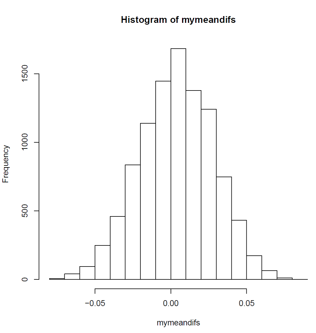
What is to be concluded? (as well conclusion as argument must be valid)

That there is significant difference between the two averages, since there are values falling to the left of -0.05 in the bootstrap distribution

That there is no significant difference between the two averages, since there are values falling to the right of 0.05 in the bootstrap distribution

That there is a clear significant difference between the two averages, since 0 obviously roughly is in the center of the bootstrap distribution

That there is no significant difference between the two averages, since 0 obviously roughly is in the center of the bootstrap distribution

The data comes from two different normal distribution

02402 · Test Quiz 13

Question 1 of 13

Question 2 of 13

Question 3 of 13

Question 4 of 13

Question 5 of 13

Question 6 of 13

Question 7 of 13

Question 8 of 13

Question 9 of 13

Question 10 of 13

Question 11 of 13

Question 12 of 13

Question 13 of 13